How Many EEG Channels Do You Actually Need for Classification?

Sensor Reduction and Generalization

Machine-learning pipelines often begin with a simple assumption: if more measurements are available, more measurements should be used. That assumption is especially expensive in sensor-based systems. Every additional EEG channel adds another electrode, another signal stream, another source of setup complexity, and another feature block that must be processed at inference time.

The present work builds on the methodology used in previous work, which examined the effects on EEG classifier performance when entire participants are held out from training data and used only for testing. That work revealed the great importance of the validation method on performance results. Now that the methodology has been established, the next step takes a more applied approach: the model must generalize to completely unknown participants. The question is how many of the original 19 EEG channels are actually needed.

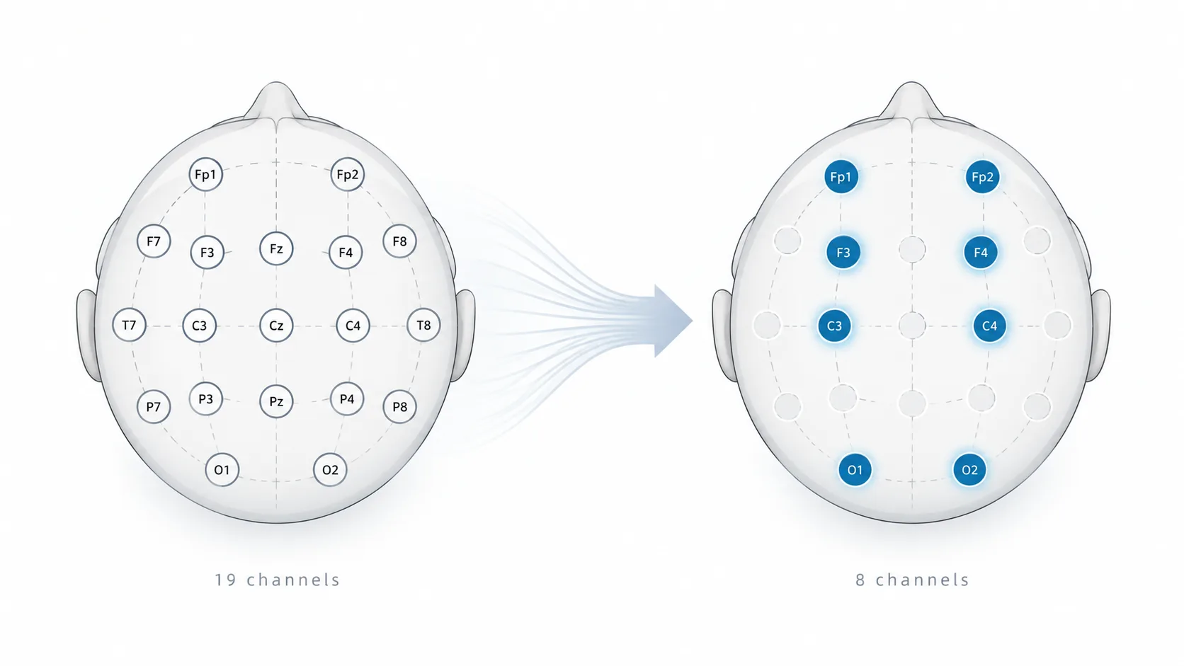
This analysis tests whether all 19 scalp EEG channels in a public mental-arithmetic dataset are necessary for cross-participant classification. The original 19-channel representation was reduced to 12, 8, 4, 2, and 1 channels while preserving the same preprocessing pipeline, spectral features, model families, and participant-held-out evaluation. The central question was practical: how much predictive performance is retained as the sensor count falls?

The first result was straightforward. Large reductions in channel count produced relatively small changes in unseen-participant performance. The second result was more informative. Several electrodes ranked near the top in nearly every training fold, yet those apparently important channels did not outperform randomly selected channel subsets when tested on held-out participants. The experiment therefore became less about identifying a supposedly optimal EEG montage and more about a broader machine-learning problem: stable feature importance does not necessarily imply better out-of-sample usefulness.

Dataset and Feature Extraction

The analysis used the EEG During Mental Arithmetic Tasks (EEGMAT) dataset from PhysioNet [1, 2]. The dataset contains 36 participants, each with one background recording and one recording collected during a serial mental-arithmetic task, for 72 EDF files in total. The classification target is the recording condition — background versus mental arithmetic — rather than a validated universal measure of cognitive load.

Nineteen scalp EEG channels were retained: Fp1, Fp2, F3, F4, F7, F8, T3, T4, C3, C4, T5, T6, P3, P4, O1, O2, Fz, Cz, and Pz. The ear-reference difference channel and ECG channel were excluded. Signals were filtered from 1 to 40 Hz and divided into non-overlapping four-second windows.

Power spectral density was estimated with Welch’s method [3]. For every channel and window, relative power was computed in four bands: theta (4–8 Hz), alpha (8–13 Hz), beta (13–30 Hz), and low gamma (30–40 Hz). Each channel contributed four features, producing 19 × 4 = 76 features per window.

The final feature matrix contained 2,134 windows: 1,594 background windows and 540 arithmetic windows across 36 participants. No NaN or infinite feature values were present. This compact, interpretable representation was intentionally kept fixed throughout the channel-reduction experiment so that changes in performance could be attributed to sensor count and channel selection rather than to changing feature engineering.

Participant-Held-Out Evaluation

Windowed EEG data consists of many observations but only a small number of individual subjects. Random division can lead to assigning windows of the same subject to both train and test sets, which is not appropriate when the goal is to estimate model performance on new individuals. All model evaluations therefore used six folds of GroupKFold cross-validation with participant ID as the grouping parameter, meaning six participants served as test data in each iteration. No test participant’s windows were used for training, normalization, or channel selection.

Three families of models were considered: weighted-class logistic regression, SVM with a radial basis function (RBF) kernel, and a weighted-class random forest of 300 trees. Both logistic regression and SVM used StandardScaler in their pipeline. The main metric was balanced accuracy, which accounts for the imbalance in the number of windows across conditions. ROC-AUC was used as an additional ranking metric.

Leakage-Safe Channel Ranking

Channel selection introduces an additional problem for the validation procedure. If channel selection is performed using all participants before cross-validation, the held-out participants would influence the selected features, making it impossible to estimate performance on truly unseen individuals. Channel selection was therefore performed separately for each training fold.

For each participant and each spectral feature, the mean background value was subtracted from the mean arithmetic value. The difference was summarized by the absolute mean of those differences normalized by their standard deviation. Four band scores for each electrode were averaged to produce a single channel score. Larger scores correspond to larger and more consistent condition differences.

Formally, for participant s and feature f, the condition difference is Δ(s, f) = mean(arithmetic) − mean(background). The feature score is |mean(Δf)| / SD(Δf). This procedure prevents participants with a large number of background windows from dominating channel selection simply due to their window count.

Performance Across Channel Counts

The primary experiment compared 19, 12, 8, 4, 2, and 1 selected channels under the same six participant-held-out folds. The resulting performance curves were flatter than expected, particularly between 19 and 8 channels.

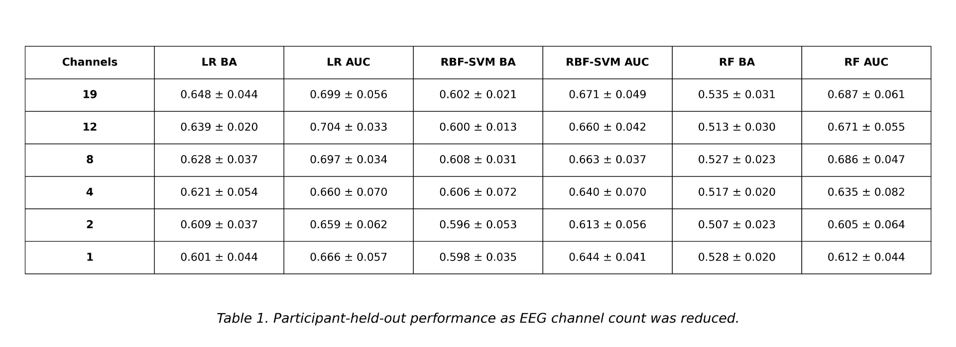
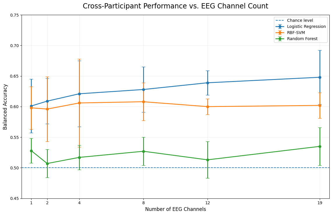
Logistic regression declined from 0.648 balanced accuracy with all 19 channels to 0.628 with eight channels, a difference of 0.020. Its AUC changed from 0.699 to 0.697. The RBF-SVM did not show a monotonic relationship between channel count and performance: balanced accuracy was 0.602 with 19 channels and 0.608 with eight. Random forest remained much closer to chance in balanced accuracy, but its eight-channel AUC of 0.686 was almost identical to the 19-channel AUC of 0.687.

Eight channels represent only 42% of the original 19-channel sensor set, corresponding to a 58% reduction in electrode count. The results do not establish eight channels as a universal optimum, but they do show that for this dataset and spectral representation, using every available channel was not required to preserve most of the observed cross-participant performance.

Channel Selection Stability

The training-only rankings were also examined across folds. Despite each fold using a different set of training participants, several channels repeatedly appeared near the top. Pz had a mean rank of 2.00 and appeared in the top four in all six folds. P4, Fz, F4, P3, and O1 also appeared in the top eight in every fold.

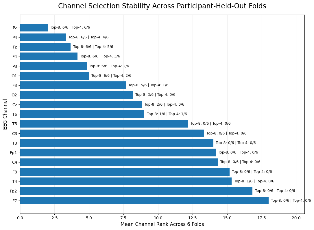
This stability initially suggested a straightforward interpretation: perhaps a small set of electrodes carried most of the useful information. That conclusion required a control. A stable ranking is only valuable if the channels it selects generalize better than reasonable alternatives.

Random-Channel Control

A random-channel baseline was added using logistic regression. For each held-out fold, random channel subsets of the same size were sampled and evaluated using identical training and test participants. An initial baseline averaged 50 random subsets per fold. Mean balanced accuracy was 0.644 for eight channels, 0.635 for four, 0.629 for two, and 0.616 for one. These values were not lower than the training-ranked subsets; in fact, they were slightly higher at every tested channel count.

A second analysis sampled 200 random subsets per fold and measured where the ranked subset fell within each fold-specific random distribution. If the ranking method consistently identified unusually strong subsets, the ranked solution should have appeared well above the 50th percentile. It did not.

Training-ranked channel subsets did not outperform the random-channel baseline. Percentile labels show the mean position of the ranked subset within the fold-specific random-subset distributions.

The result changes the interpretation of the channel-stability findings. Pz, P4, Fz, F4, P3, and O1 were consistently favored by the participant-level effect-size statistic, but that consistency did not translate into a measurable generalization advantage on unseen participants. The ranking was stable according to its own criterion without being demonstrably superior for the downstream classifier.

Interpretation of the Findings

The more important observation here is not that some electrodes are irrelevant, but that feature importance and predictive utility are two different quantities. Feature importance can be high — with large and consistent differences between conditions for a single feature — while that same feature provides minimal additional information because many correlated features already capture it. Conversely, a feature with a relatively small marginal effect can become informative through its interactions with other features.

One possible explanation for the flat channel-count curve is redundancy. Information about the spectral properties of the recording condition may be dispersed across several scalp positions, so multiple channel subsets can produce equally effective decision boundaries. This explanation fits the random-subset result well, though the current experiment cannot identify the physiological mechanism behind the phenomenon.

A further possibility is that the ranking criterion is incompatible with the learning algorithm. The channel score ranks the consistency of participants’ condition differences for each feature individually and then sums those scores within each electrode. Logistic regression and RBF-SVM, however, optimize decision boundaries in a multivariate fashion, so a univariate ranking criterion may not align well with what these models actually exploit.

Implications for Sensor-Based Machine Learning

The channel-count result and the channel-ranking analysis together point to a broader lesson for sensor-based machine learning. Reducing sensor count aggressively — by more than half in this case — need not substantially harm cross-participant generalization when the feature representation is compact and the information is distributed across the sensor array. At the same time, stable feature importance scores derived from training data should not be treated as a reliable guide to which sensors matter most for unseen subjects. Validating any selection strategy against a random baseline is a practical and informative check that is straightforward to implement and easy to overlook.